ML-HW2 PDF
Update on October 19, 2019: ML-HW2 Solution PDF
Question 1

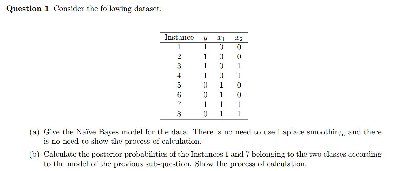
(a) Considering Naive Bayes model, the features are conditionally independent. And because of the binary features, we can use Bernoulli distribution for the class-conditional probability
$$ p(\vec{x}|y=c) = \prod_{j=1}^2Ber(x_j|\mu_{jc}) $$
Use Bayes rules, the posterior probability
$$ \begin{aligned} p(y=c|\vec{x}) &= \frac{P(\vec{x},y=c)}{P(\vec{x})} \\ &= \frac{P(y=c)}{P(\vec{x})} \cdot p(\vec{x}|y=c) \\ &= \frac{P(y=c)}{P(\vec{x})} \cdot \prod_{j=1}^2Ber(x_j|\mu_{jc}) \end{aligned} $$
(b) For instance 1, $\vec{x}=\{x_1,x_2\}=\{0,0\}$
$$ P(\vec{x},y=0) = P(y=0) \cdot Ber(x_1|\mu_{10}) \cdot Ber(x_2|\mu_{20}) = \frac{3}{8} \times 0 \times \frac{2}{3} = 0 $$
$$ P(\vec{x},y=1) = P(y=1) \cdot Ber(x_1|\mu_{11}) \cdot Ber(x_2|\mu_{21}) = \frac{5}{8} \times \frac{4}{5} \times \frac{2}{5} = \frac{1}{5} $$
$$ \therefore P(\vec{x}) = 0 + \frac{1}{5}=\frac{1}{5} $$
$$ p(y=0|\vec{x}) = \frac{P(\vec{x},y=0)}{P(\vec{x})} = \frac{0}{1/5} = 0 $$
$$ p(y=1|\vec{x}) = \frac{P(\vec{x},y=1)}{P(\vec{x})} = \frac{1/5}{1/5} = 1 $$
For instance 7, $\vec{x}=\{x_1,x_2\}=\{1,1\}$
$$ P(\vec{x},y=0) = P(y=0) \cdot P(\vec{x}|y=0) = P(y=0) \cdot Ber(x_1|\mu_{10}) \cdot Ber(x_2|\mu_{20}) = \frac{3}{8} \times 1 \times \frac{1}{3} = \frac{1}{8} $$
$$ P(\vec{x},y=1) = P(y=1) \cdot Ber(x_1|\mu_{11}) \cdot Ber(x_2|\mu_{21}) = \frac{5}{8} \times \frac{1}{5} \times \frac{3}{5} = \frac{3}{40} $$
$$ \therefore P(\vec{x}) = \frac{1}{8} + \frac{3}{40} = \frac{1}{5} $$
$$ p(y=0|\vec{x}) = \frac{P(\vec{x},y=0)}{P(\vec{x})} = \frac{1/8}{1/5} = \frac{5}{8} $$
$$ p(y=1|\vec{x}) = \frac{P(\vec{x},y=1)}{P(\vec{x})} = \frac{3/40}{1/5} = \frac{3}{8} $$
Question 2

If all classes shares the same covariance matrix
$$ \begin{aligned} P(y=c|\vec{x}) & \propto P(y=c) \cdot P(\vec{x}|y) \\ & \propto \pi_c \cdot e^{-\frac{(\vec{x}-\vec{\mu_c})^T \cdot \Sigma^{-1} \cdot (\vec{x}-\vec{\mu_c)}}{2}} \\ &= \pi_c \cdot e^{-\frac{1}{2}\vec{x}^T\Sigma^{-1}\vec{x}} \cdot e^{\frac{1}{2}\vec{\mu_c}^T\Sigma^{-1}\vec{x} - \frac{1}{2}\vec{\mu_c}^T\Sigma^{-1}\vec{\mu_c}} \\ & \propto e^{\vec{\mu_c}^T\Sigma^{-1}\vec{x} - \frac{1}{2}\vec{\mu_c}^T\Sigma^{-1}\vec{\mu_c} + log\pi_c} \end{aligned} $$
Let $\vec{w_c}^T=\vec{\mu_c}^T\Sigma^{-1}$ and $b_c=-\frac{1}{2}\vec{\mu_c}^T\Sigma^{-1}\vec{\mu_c} + log\pi_c$. Then
$$P(y=c|\vec{x}) \propto e^{\vec{w_c}^T\vec{x}+b_c}$$
According to the above analysis, if all classes shares the same covariance matrix, the GDA goes back to softmax regression. And if let $C=2$, we can get the logistic regression model.
| Comparision | Logistic Regression | GDA |
|---|---|---|
| Distribution of Data | $P(y=c \mid \vec{x},\vec{w})=Ber(y\mid \sigma(\vec{w}^T\vec{x}))$ . It's a weaker assumption but performs more robust. It's a simpler and lower-lever model. | $P(\vec{x}\mid y=c)= N(\vec{x}\mid \vec{\mu},\vec{\Sigma})$. It is a stronger assumption but may not be reliable when encountering some extreme situations. |
| Amount of Data | It requires more data so it's harder for training. | It requires less data to achieve a certain level of performance than logistic regression. It's easier to learn parameters. |
Question 3

The logistic regression is a kind of dicriminative model and the GDA is a kind of generative model. When we come to the topic of classification, we have other kinds of classifiers. For example, on the one hand, Naive Bayes classifier, Bayesian networks, LDA and etc. belong to generative model. On the other hand, SVM, Softmax, decision tree, neural network. The comparision of generative classifiers and discriminative classifiers is as follows:
| Comparision | Generative Classifier | Discriminative Classifier |
|---|---|---|
| Parameter Estimation | Generative classifier finds the best class the object belongs to by maximizing the joint probability $P(\vec{x}, y)$ using $P(y)$ and $P(\vec{x}\mid y)$. It's easier to do this because it has closed-form formulae for MLE | Discriminative classifier directly do classificaton by maxizing the conditional probability $P(y\mid \vec{x})$. More complex to do parameter estimation because it requires gradient descent to compute MLE |
| Missing Data | No principled way to handle | EM algorithm |
| Features Transform | Hard because the new feature are correlated in complex ways | Easy. $\vec{x} \rightarrow \Phi(\vec{x})$. Used in deep learning. |
| Semi-supervised Learning | Can use unlabeled data to help with training | Harder |
Question 4


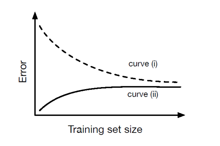
The curve(ii) represents the training error. On the one hand, this is because that generally the test error will be larger than training error. On the other hand, when the training data set is small, the data set cannot well illustrate the nature of the whole data. It's easy to train a model with zero training error but very high test error. When gradually increasing the trainning set, the training error would increase from zero to a stable value and the test error would decrease from a large value to the stable value.
The gap is called generalization gap. According to VC Theorem, I use $m$ to represent the sample size and $d=VC(H)$ to represent the model complexity. The gap between training error $\hat{\epsilon}(h)$ and test error $\epsilon(h)$ satisfies an inequality relation as follows:
With probability at least $1-\delta$, we have that all for $h\in H$
$$ |\epsilon(h)-\hat{\epsilon}(h)| \leq O \left( \sqrt{\frac{d}{m}log\frac{m}{d}+\frac{1}{m}log\frac{1}{\delta}} \right) $$

In general, we have $\frac{m}{d}>e$ so in the interval $[e,+\infty]$
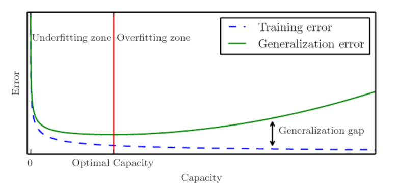
- Fixing m. $d$ increases $\rightarrow$ $\frac{m}{d}$ decreases $\rightarrow$ $\frac{d}{m}log\frac{m}{d}$ increases $\rightarrow$ $O(\cdot)$ increases $\rightarrow$ generalization gap widens. i.e. When increasing the model complexity, the geralization gap would widen. Their relationship can be further illustrated by figure 2. As we see, the gap between green line and blue line is getting bigger and bigger as the model capacity increases.
- Fixing d. $m$ increases $\rightarrow$ $\frac{m}{d}$ increases $\rightarrow$ $\frac{d}{m}log\frac{m}{d}$ decreases $\rightarrow$ $O(\cdot)$ decreases $\rightarrow$ generalization gap narrows. i.e. The generalization gap narrows as the sample size becomes larger. And this is already shown in figure 1. Hence, more data implies better performance of learning an algorithm.
本博客文章除特别声明外,均可自由转载与引用,转载请标注原文出处:http://www.yelbee.top/index.php/archives/178/
